Matrix similarity and eigenvalues

Introduction

Recently I was reading Data Science from Scratch by Joel Grus. One of Grus’ prerequisites for doing data science is linear algebra. I took a linear algebra course as a freshman but I didn’t do particularly well in it and what little I learned I’ve long since forgotten. So I’ve decided to brush up on my linear algebra by working through a textbook called Linear Algebra by Jim Hefferon, a free online text book recommended by Grus.

In the fifth and final chapter of Linear Algebra the author’s program is to come up with a kind of normal form of matrices that would become an equivalence class for matrices. The chapter starts by introducing the notion of matrix similarity. If two matrices are similar then they essentially are the same transformation, just in different bases.

The normal form the chapter builds to is the Jordan normal form. There are matrices that are diagonalizable and for these matrices a diagonal matrix is the normal form (more on this later). But not all matrices are diagonalizable. Some are nilpotent. A nilpotent matrix is one that when applied to itself multiple times eventually becomes the zero matrix. The canonical form of nilpotent matrices is all zeros and some ones on the sub-diagonal. Jordan normal form essentially combines these two canonical forms to create a canonical form that can represent any matrix.

That’s about all I want to say about Jordan normal form. Here I’ll be focusing on diagonalizability and how to compute eigenvalues and eigenvectors.

Diagonalizable matrices

I introduced matrix similarity by saying that similar matrices represent the same transformation just in different bases. More formally, two matrices, $A$ and $B$ are similar if there exists a matrix $P$ such that $A = P B P^{-1}$ . This $P$ matrix is a basis conversion matrix and converts from B’s basis to A’s basis; the inverse converts in the opposite direction.

A diagonal matrix is defined as a matrix that is all 0’s except for non-zero entries on the diagonal. A matrix $T$ is diagonalizable if there is a matrix $P$ such that $P T P^{-1}$ is a diagonal matrix. So the diagonal representation of $T$ is similar to $T$ and any matrix that is similar to $T$ is also similar to the diagonal representation of $T$ . Later we’ll see how to determine if a matrix is diagonalizable.

Let’s think a little bit about what a diagonal matrix represents. Let’s say we have a diagonal matrix $T$ with $n$ rows and columns. $T$ is a matrix with all zeroes except that in the i-th row there is a diagonal entry that we’ll call $\lambda_i$ . The basis of the domain and codomain is the same and the vectors that make up this basis we’ll call $\beta_i$ . Then, for each basis vector:

$ T \beta_i = \lambda_i \beta_i $

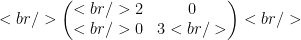
Let’s look at an example. Let T be the following diagonal 2×2 matrix with the natural basis:

$ \begin{pmatrix} 2 & 0 \cr 0 & 3 \end{pmatrix} $

So for $T$ , $\lambda_1 = 2$ , $\lambda_2 = 3$ , $\beta_1 = (1, 0)$ and $\beta_2 = (0, 1)$ . We can easily show that $T \beta_1 = \lambda_1 \beta_1$ :

$ \begin{pmatrix} 2 & 0 \cr 0 & 3 \end{pmatrix} \begin{pmatrix} 1 \cr 0 \end{pmatrix} = \begin{pmatrix} 2 \cr 0 \end{pmatrix} = 2 \begin{pmatrix} 1 \cr 0 \end{pmatrix} = \lambda_1 \beta_1 $

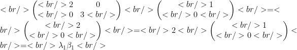
And likewise for $\lambda_2$ and $\beta_2$ .

For a diagonal matrix, we’ll call the $\lambda_i$ the eigenvalues and the $\beta_i$ the eigenvectors. If we can develop a way to compute the eigenvalues and their associated eigenvectors for a matrix then we can construct the diagonal representation of a matrix which would simply have the $\lambda_i$ as the diagonal entries and the basis would be the eigenvectors.

Computing Eigenvalues and Eigenvectors

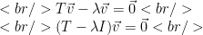
So how do we find eigenvalues? What we’ll do is solve for $T \vec{v} = \lambda \vec{v}$ . This becomes

$ T \vec{v} - \lambda \vec{v} = \vec{0} \\ (T - \lambda I) \vec{v} = \vec{0} $

$(T - \lambda I) \vec{v} = \vec{0}$ is a homogeneous system and the only solution for $\vec{v}$ is $\vec{0}$ if $T - \lambda I$ is nonsingular. (A nonsingular matrix is one that has a unique solution but for a homogeneous system the only unique solution is $\vec{0}$ ). That’s not what we want; we want non-zero solutions for $\vec{v}$ . That will only happen if $T - \lambda I$ is singular, which is true when $|T-\lambda I| = 0$ , that is, when the determinant of $T - \lambda I$ is 0.¹ This equation, $|T-\lambda I| = 0$ is called the characteristic equation.

Let’s look at an example. Let $T$ be

$ \begin{pmatrix} 3 && 0 \cr 8 && -1 \end{pmatrix} $

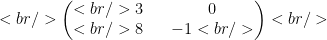
Then

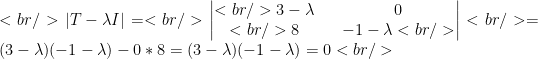
$ |T - \lambda I| = \begin{vmatrix} 3 - \lambda && 0 \cr 8 && -1 - \lambda \end{vmatrix} = (3 - \lambda) (-1 - \lambda) - 0 * 8 = (3-\lambda)(-1-\lambda)= 0 $

This equation has two solutions, $\lambda = -1, 3$ . (Note: computing a determinant for a matrix of dimension 2 is relatively simple. To compute a determinant in higher dimensions see Laplace’s expansion.)

For each eigenvalue we can find a corresponding set of eigenvectors. Let’s start with the eigenvalue -1. We want to find vectors for which $T\vec{v} = -1\vec{v}$ .

$ \begin{pmatrix} 3 && 0 \cr 8 && -1 \end{pmatrix} \begin{pmatrix} a \cr b \end{pmatrix} = -1 \begin{pmatrix} a \cr b \end{pmatrix} $

This becomes the following set of equations:

$ 3a = -a \\ 8a - b = -b $

The only solution for the first equation is $a = 0$ . The second equation then reduces to $b=b$ which has an infinite number of solutions. Therefore the following is the set of eigenvectors for eigenvalue $-1$ .

$ \lbrace \begin{pmatrix} 0 \cr b \end{pmatrix} | b \in \mathbb{R} \} $

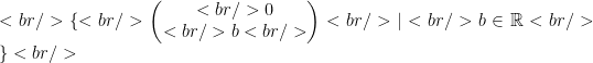
This last is called an eigenspace. We can use any non-zero vector from this space to be an eigenvector, for example if we want to get a basis vector.

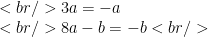
Similarly, plugging in the eigenvalue 3 yields

$ 3a = 3a \\ 8a - b = 3b $

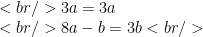
The first equation has an infinite number of solutions. The second equation reduces to $b = 2a$ . Therefore the following is the set of eigenvectors for the eigenvalue 3.

$ \lbrace \begin{pmatrix} a \cr 2a \end{pmatrix} | a \in \mathbb{R} \} $

So the diagonal representation of $T$ is

$ \begin{pmatrix} -1 && 0\cr 0 && 3 \end{pmatrix} $

We can choose two eigenvectors, corresponding in order with the eigenvalues in the above matrix, to make up the basis:

$ \langle \begin{pmatrix} 0 \cr 1 \end{pmatrix}, \begin{pmatrix} 1 \cr 2 \end{pmatrix} \rangle $

Now that we can compute eigenvalues we can easily determine if a matrix is diagonalizable: a matrix of dimension n is diagonalizable if it has n distinct eigenvalues because we can use those eigenvalues to make up the diagonal entries of the matrix and the eigenvectors associated with them make up the basis. Let $P$ be the matrix whose column vectors are these basis vectors. Then the diagonalization of $T$ is $\hat{T}$ :

$ \hat{T} = P^{-1} T P $

Conclusion

Now we can not only determine if a matrix is diagonalizable but also produce the diagonal representation of a matrix and its basis. Why would we want to diagonalize a matrix? For a diagonalizable matrix, the diagonal representation is the easiest to work with. One example of how diagonal matrices are easier to work with is matrix exponentiation. If you have a diagonal matrix $T$ with diagonal entries $\lambda_i$ then $T^n$ is a diagonal matrix with diagonal entries $\lambda_i^n$ . Thus $T^n$ is very easy to compute. If on the other hand $T$ isn’t diagonal but it is diagonalizable, and $\hat{T}$ is the diagonal representation of $T$ , then $T^n$ is

$ (P\hat{T}P^{-1})(P\hat{T}P^{-1})...(P\hat{T}P^{-1}) = P \hat{T^n} P^{-1} $

Since computing $\hat{T^n}$ is very simple, it is worth it to transform into its basis and back again as a way of computing $T^n$ .

In addition to practical applications can we also develop an intuition about eigenvectors from the preceding discussion? Since a linear transformation applied to an eigenvector doesn’t change its direction, the eigenvectors of a linear transformation can be thought as “axes” of the linear transformation. We can see that from how the eigenvectors of a matrix are used to form the basis vectors for the diagonal representation. The associated eigenvalues can be thought of as the amount of “skew” along those axes that the linear transformation imparts to vectors to which it is applied. So in a sense the eigenvectors and eigenvalues describe the action of a linear transformation on vectors to which it is applied, and this description appears to be as succinct as possible.

Why is a matrix singular if the determinant is 0? Recall that singular matrices do not have a unique solution. One way to determine if a matrix is singular is to reduce it via Gaussian elimination to echelon form. If the result does not have leading coefficients for each row then it will not have a unique solution. But if it is missing a leading coefficient in one row then it must have a zero on that diagonal entry. One way to compute a determinant is to reduce a matrix to echelon form and then take the product of the diagonal entries. So the determinant will be 0 only if there is a 0 on the diagonal which happens when there is a missing leading coefficient. ↩

Matrix similarity and eigenvalues

Introduction

Diagonalizable matrices

Computing Eigenvalues and Eigenvectors

Conclusion

Like this:

Leave a comment

Leave a Reply Cancel reply

Introduction

Diagonalizable matrices

Computing Eigenvalues and Eigenvectors

Conclusion

Share this:

Like this:

Leave a comment

Leave a Reply Cancel reply